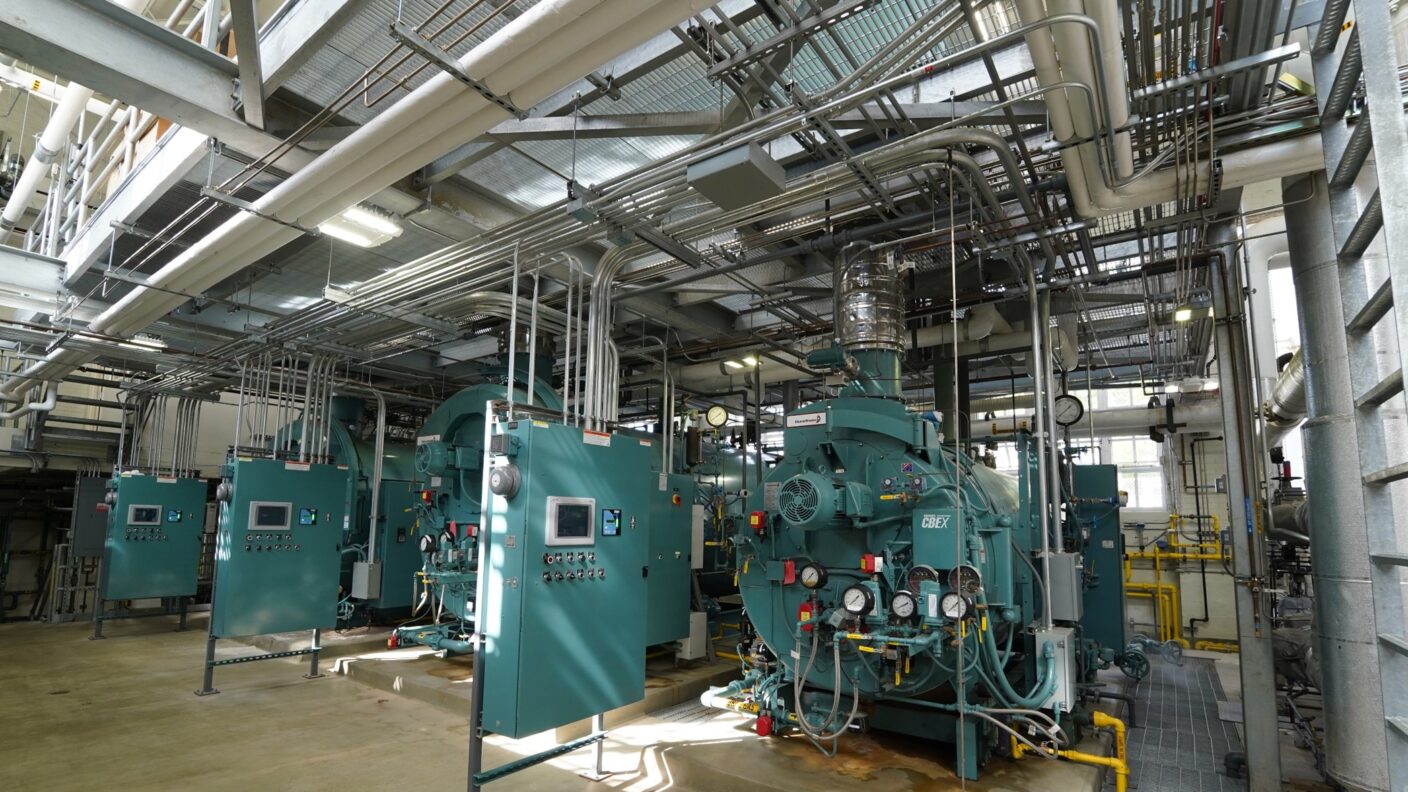
CASE STUDY: Compressible Fluid Analysis Applications: Campus Steam Networks

Learning Objectives

After reading this case study, you should be able to:

1. Determine the difference between compressible and incompressible flow.
2. Understand the challenges associated with modeling flow in compressible fluid systems.
3. Identify when compressible flow can be analyzed or modeled with simple approaches versus advanced software.

Project Description

Fluids in most heating, ventilation, and air conditioning (HVAC) systems are typically either a gas (compressible fluid) or a liquid (incompressible fluid). In order to determine pipe sizes and pressure drops for these fluids, the flow must first be analyzed. Sometimes compressible fluids can be analyzed assuming incompressible flow.

Is it appropriate to model a low-pressure steam system as incompressible flow? As we will discuss in this case study, it’s usually acceptable in HVAC applications; however, depending on project complexity and specific Owner requirements, doing so may cause an oversimplification in the system modeling and provide challenges for accurate recommendations.

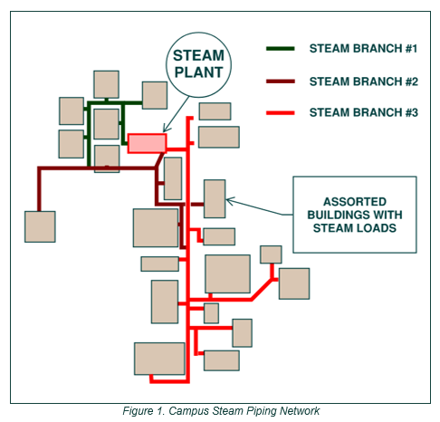
Let’s consider a recent project where Systems West performed a pre-design analysis for a large university client located in the Pacific Northwest. The University maintains a buried steam piping system serving a campus of assorted academic, office, and dormitory buildings. This complex steam system network contains thousands of feet of steam piping comprised of three branches from the steam plant, interconnected as shown in the schematic diagram in Figure 1.

With failures occurring at several current locations in the distribution system and a planned campus expansion occurring over the next several years, the University sought to understand how much of the piping needed to be resized in order to serve the heating loads of all existing and future buildings. The system is low-pressure steam operating at about 12 psig at the central steam plant, and the University’s project requirements only allowed for a 3.5 psi total pressure drop at the minimum pressure in the main.

Due to the complex network of interconnected piping and the tight pressure loss requirements, accuracy of the steam system model was vital to provide actionable recommendations. This also raised the questions of whether it is reasonable to model systems containing compressible fluid (e.g., steam) as incompressible flow, and when it is required to account for compressibility.

Flow Analysis Method

Engineers analyze fluid flow by modeling the flow as either a compressible flow or an incompressible flow in order to determine pressure losses and appropriate pipe sizes. In the case of our University example, a flow analysis of the steam distribution system is required to determine the proper piping size for the planned campus expansion. This analysis becomes more complex when there is substantial interconnected piping and when the fluid medium needs to be modeled as compressible flow. To help illustrate this, let’s first look at the following equations that govern the analysis for fluid flow in a piping system for both compressible and incompressible fluids.

The application of these equations in a flow analysis depends on whether the fluid is treated as incompressible or compressible.

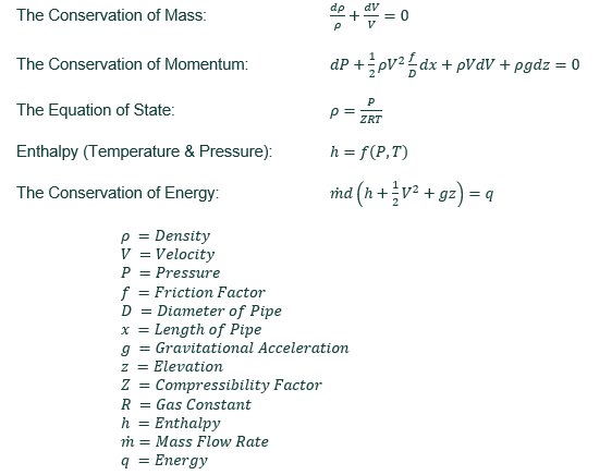
Incompressible fluids typically have negligible changes in density when external pressures or temperatures fluctuate; therefore, the volume changes are nearly zero and there is virtually no change from the Equation of State. When modeling a fluid as incompressible flow, many of the factors in the above equations go to zero and calculations for simple pipe systems become easier, though complex networks may still be difficult to analyze without software. Examples of incompressible fluids we often see in MEP systems are:

✔ Water
✔ Oil
✔ Glycol

Compressible fluids experience a change in density as a result of an external pressure acting on the fluid or changes in temperature. When density changes, we know from the Conservation of Mass equation that the volume will change inversely. From the Equation of State, if a system is near adiabatic (negligible temperature changes), a decrease in pressure decreases the density and the volume must increase. When modeling a fluid as compressible flow, the above equations are dependent upon each other, and spreadsheet calculations become complicated, especially with a network of interconnecting pipes. Examples of compressible fluids we often see in MEP systems are:

✔ Steam
✔ Air
✔ Natural Gas
✔ Propane
✔ Nitrogen
✔ Oxygen

Modeling Compressible Flow as Incompressible

Sometimes, a compressible fluid system can be modeled as incompressible flow to help simplify calculations. This is often the case when analyzing airflow in ductwork, for example. Two common rules of thumb are used to help determine if a system containing a compressible fluid can be analyzed as incompressible flow:

M <0.3 (Mach number is less than 0.3)
P _in – P _out <10% P _in (Pressure in section analyzed drops less than 10%)

These are only general guidelines, however, and must be combined with good engineering judgment for final determination. The following tables show a comparison of results obtained by analyzing incompressible fluid systems as compressible versus incompressible flow and how the accuracy of results may be influenced.
Table 1 shows an analysis of a compressed air flow. The Mach number (velocity of fluid divided by the speed of sound in the fluid) was less than 0.3. The pressure drop at the end of the pipe was greater than 10% of the inlet of the pipe. Analyzing the flow as incompressible resulted in a calculated pressure drop of 15.95 psi. Analyzing the flow as compressible provided a marginally more accurate result with a pressure drop of 17.53 psi. In most scenarios, this difference is negligible, and it would be appropriate to assume the compressed air system as incompressible flow even though it didn’t pass the criteria listed above. However, if there are several similar sections of pipe to be added together, an engineering judgment will be required depending on the end of line pressure requirements.

Table 2 is an example of a length of pipe used for the distribution of natural gas inside a city gate from a utility company. The length of pipe in this section is long and the pressure drops are significant. Again, the Mach number is less than 0.3 for this section of pipe, and the pressure drop is significantly higher than 10% of the inlet pressure. In this example, the incompressible analysis is clearly not acceptable compared to the actual losses calculated with a compressible flow analysis. The incompressible flow analysis shows an ending velocity of 145 ft/s with a pressure drop of 24.02 psi. The more accurate compressible flow calculation has the ending pipe velocity of 347 ft/s with a pressure drop of 34.76 which is 140% of the pressure losses calculated as incompressible. Clearly, analyzing a system as a compressible flow is necessary in cases such as this.

Our Approach

HVAC applications of compressible flow, such as air-in-duct systems and simple low-pressure steam systems, are typically modeled as incompressible flow; however, the complex network of interconnected piping and the tight pressure loss requirements of the University’s campus steam distribution required our team to consider analyzing the system as compressible flow.

Figure 2 below illustrates the analysis of a section of the campus distribution assuming incompressible flow.

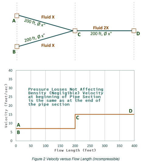
In the top half of Figure 2, the same fluid (low-pressure steam) flows in the same diameter pipe for the same distance from points A to C and from B to C. Pipe CD is the same size and length as pipes AC and AD but carries twice the volume.

In the bottom half of Figure 2, the graph shows an example of an incompressible fluid’s velocity versus system length. The fluid’s pressure continues to decrease with the increased velocity at point C; however, with an incompressible fluid, the substantial changes in pressure due to frictional pressure losses have little effect on the density or volume. Therefore, the volumetric flowrate remains the same at the inlet and outlet of the pipes and the velocity remains constant when there are no changes in fluid or pipe size. The velocity from points A to C and B to C are flat until the fluid flow rates are combined. Likewise, once the fluids are combined at point C, the velocity increases at point C, but remains unchanged between points C and D even though the pressure on the fluid is decreasing from the frictional pressure losses.

Figure 3 below illustrates the analysis of the same section of the campus distribution assuming incompressible flow.

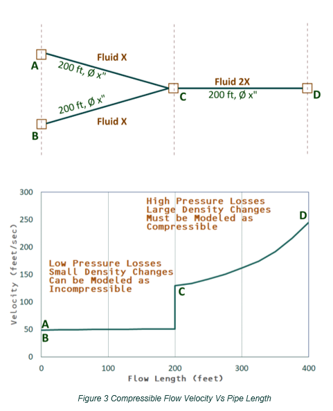
Interestingly, in this example, the flow in pipes AC and BC have a low enough velocity that the pressure losses are not significant along those pipes and the density does not change much from point A to point C, or from point B to point C. In pipes AC and BC, the fluid could be analyzed as an incompressible flow despite the fluid being compressible; however, after the flows are combined, the flow through pipe CD has a significantly higher velocity starting at point C. Since pressure losses increase with the square of the velocity, the higher velocity causes substantial pressure losses throughout pipe CD. As the fluid continues to lose pressure along the pipe, the compressible fluid continues to expand, and the velocity continues to increase as the conservation of mass and momentum are maintained from point C to point D with the decreasing density due to decreasing pressure. While the conservation of mass is maintained throughout the piping system, the change in density causes the volumetric flowrate to increase with a compressible fluid.

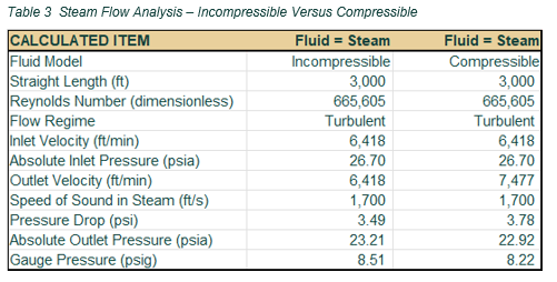
In Table 3, a simplified analysis of the University’s campus steam analysis is compared between assuming incompressible and compressible flow. This calculation does not consider fittings and branch flows. For this flow of steam, the Mach number is less than 0.3 and the pressure drop exceeds 10% of the inlet pressure of 12 psig (26.7 psia). In this example, the incompressible analysis might indicate that the pressure loss of 3.49 psi would be on the edge of being acceptable, while the more accurate compressible flow analysis clearly shows that the 3.78 psi pressure drop is not acceptable based on client requirements. Remember, the Owner’s requirement only allowed for a 3.5 psi total pressure drop at the minimum pressure in the main.

Table 3 Steam Flow Analysis – Incompressible Versus Compressible

As such, we opted to analyze the University’s steam system using a software program capable of analyzing compressible flow systems with complicated piping networks. This approach allowed for a variety of scenarios with different-sized piping and a more accurate pressure loss calculation when the allowable pressure losses were small. In the end, the analysis recommended an increase in pipe size along one of the system’s three interconnected piping loops from 10 to 12 inches in diameter.

Conclusion

Many factors play a role in approaching the analysis of piping networks with compressible fluids. Typical questions that require engineering judgment include:

✔ What is the fluid and the fluid velocity?
✔ How long is the piping distance of each section analyzed?
✔ How much tolerance is acceptable in the result?
✔ Do we expect large density differences within the pipe section?

Nearly all HVAC comfort air systems are analyzed as incompressible flows because the velocities are low enough that the change in density is negligible. Likewise, many steam and natural gas systems are small systems where the pressures and densities are also likely to be considered constant.

We recommend that if a compressible fluid is at high velocities or high pressures, or if there are long distances and complex piping, engineers should avoid incompressible assumptions when working with these compressible fluids.

Case Study Contributors: Joe Iaccarino, Dorrie Matthews, Mark Willett, Kory Bowlin

---

 Download the Case Study PDF

  Back to Our Work